
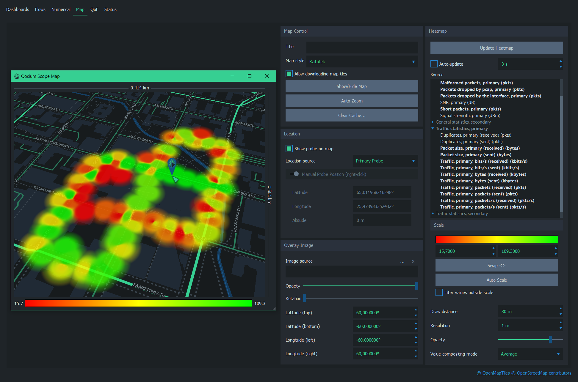
Map Tab
The map tab in the Scope workspace area is used to draw heatmaps on a geographical map. This type of visualization is beneficial when measuring Quality of Service or Quality of Experience in a real location.
Contents
1. Overview #
The map tab consists of two main elements: Map Window and Settings. See the following subsections for more information on these elements.
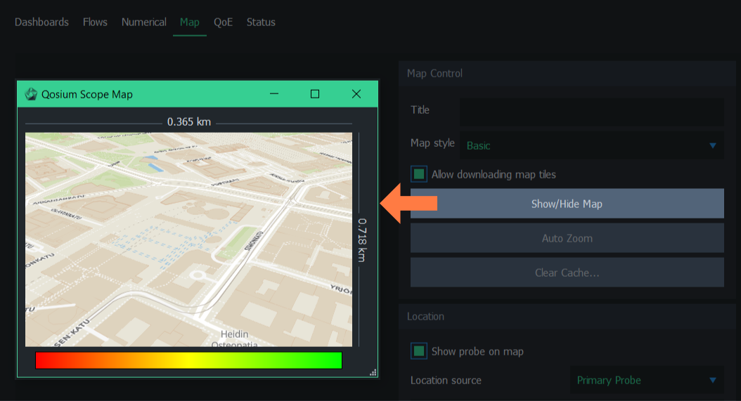
2. Map Window #
To open the map window, press Show/Hide Map in the Map Control settings group.
The window can be moved, scaled, maximized, and minimized normally as any other window. The map can be navigated with a few mouse/keyboard controls:
- Zoom in/out - Mouse wheel up/down
- Pan map - Press and hold the left mouse button and drag
- Pitch/rotate map - Press and hold either left or right Ctrl button on the keyboard, then simultaneously press and hold the left mouse button and drag
3. Settings #
The map is configured via settings displayed on the right side of the tab. See the following subsections for more information on each settings group.
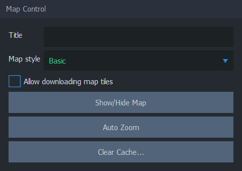
3.1. Map Control #
The map control group has controls for showing/hiding the map window, selecting map theme, and controlling map data download and caching.
When Allow downloading map tiles is checked, Scope can download map data from the map cloud service. It is recommended to keep this option checked when preparing a measurement but unchecked during measurement if there’s a risk that the traffic between Scope and map cloud service will disrupt measurement results.
Show/Hide Map toggles the visibility of the map window.
Use Auto Zoom to reset pitch and rotation. Auto-zoom also sets location and zoom according to the following priority:
- Focus on the heatmap, if available
- Focus on overlay image, if available
- If neither heatmap nor overlay image is visible, focus on the map cursor
Clear Cache… removes the map cache file from the computer. Use it to release disk space (typically ~10-60MB). Removing the cache file can be helpful when resolving issues related to map data download & rendering. Removing the map cache does not affect heatmap or measurement results.
3.2. Location #
The location group considers the geographical location of the Probes.
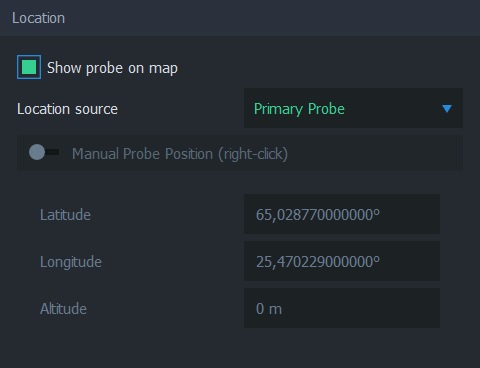
Show Probe on map toggles the visibility of the selected source Probe icon on the map. The icon appears on the map as follows:

If the Probe icon is not visible on the map even when this option is checked, it may be due to the Probe having no location info yet, or the map hasn’t been updated.
Manual Probe Position allows placing the location of the source Probe manually. This is useful functionality when you are performing, e.g., indoor measurements, where it is not possible to enable GNSS or other automatic positioning systems to Probe. During measurement, enable this option, then right-click anywhere on the map. The map cursor appears in this location. Manual positioning is available only when the measurement is running.

3.3. Overlay Image #
The overlay image can be used to add an image on top of the map. Typically, this feature is used to add a floor plan for an interior measurement or another layout image of a known location whenever the map itself is visually inadequate.
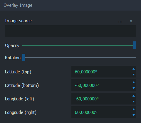
Image source indicates the filename of the current overlay image. Use … to select the image file or x to remove the current overlay image.
Opacity controls the transparency of the image. By default, the overlay image is fully opaque. Adjust the opacity to allow map visuals to pass through the overlay image partially.
Rotation allows adjusting the overlay image orientation if the source image is not aligning with the map projection.
Latitude (top), Latitude (bottom), Longitude (left), and Longitude (right) are used to align the overlay image on top of the map.
3.4. Heatmap #
The heatmap group contains controls for drawing and displaying the QoS heatmap on the geographical map.
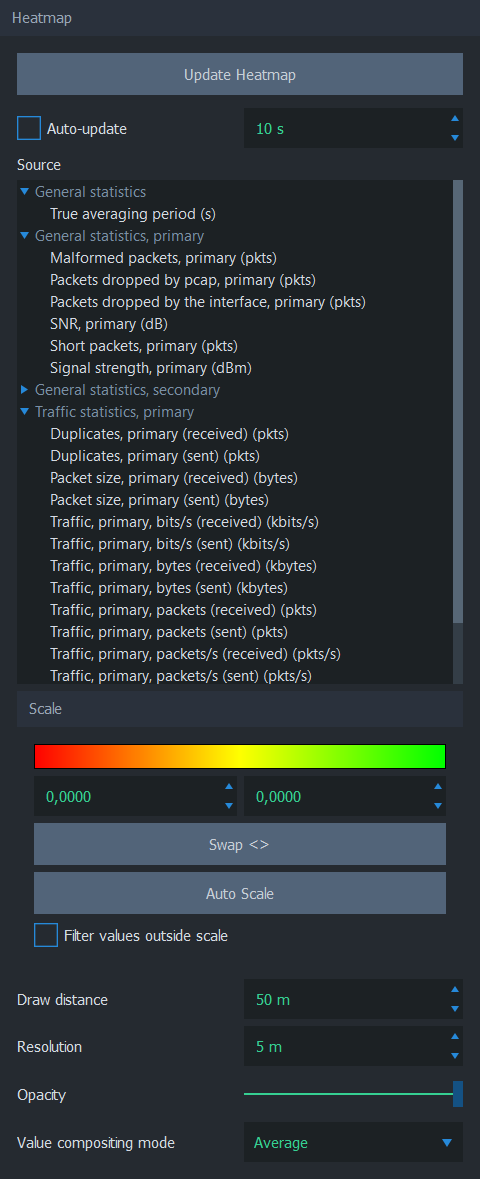
Update Heatmap, as the name implies, updates the heatmap immediately. The time the update takes depends on the amount of data and the visualization settings.
Auto-update can be used to update the heatmap in every nth second. Use the spin box to adjust the interval.
Source determines the QoS statistic that the heatmap visualizes. Use the blue triangles to expand/collapse each statistics group.
The Scale group controls how the sample values are scaled linearly into the displayed gradient. Give the scale limits manually, or use Auto Scale to automatically use the current minimum and maximum samples as scale limits. Use Swap <> to swap the given scale limits, effectively inverting the heatmap colors. When Filter values outside scale are checked, values outside scale limits are not included in the heatmap.
Draw distance indicates the radius of influence of each data point. There’s no right or wrong value for draw distance; instead, choose a value that serves the best visual appearance. For an outdoor measurement, values starting from 10 m are usually sensible. For small indoor spaces, values between 1 and 10 meters make more sense.
Resolution determines the draw precision of the heatmap image. Low-resolution values yield more accurate images than higher values. Keep in mind that the heatmap’s actual precision depends on the amount and distribution of the measurement samples.
Opacity controls the transparency of the heatmap. By default, the heatmap is fully opaque. Adjust the opacity to allow map visuals to pass through the heatmap partially.
Value compositing mode determines the method of resolving the value of overlapping samples. Overlapping samples occur when two or more measurement samples are taken from the same location. The options are:
- Average - Calculate the average of the samples
- Worst value - Take the worst value and visualize it
- Best value - Take the best value and visualize it